Warning
The tutorial is still in the process of being finalized.
Simulation workflow with The Virtual Brain
Disclaimer
The methods and software used in this tutorial have not been certified for clinical practice and should be considered for research purposes only.
Requirements
There are no technical requirements to follow this tutorial because the dataset and software are available on the HIP.
HIP software used in this tutorial:
HIP dataset used in this tutorial:
“tvb-preprocessed-tutorial-data” located in the shared tutorial_data folder.
Prepare the working environment
This tutorial requires to use The Virtual Brain, which is available on the HIP, and it is advised to initiate a new Desktop. Please, refer to the How to use Desktops and run applications from the App Catalog guide if you need help with this step.
Simulation workflow
Jupyter Notebook
Once The Virtual Brain app has started, you can view this tutorial in the form of an interactive Jupyter Notebook by double clicking the file named “simulation.ipynb” in the left sidebar.
Here we will show a short demonstration of using data from HIP partners to do simulation, with parameters guessed from one of the patient’s seizures.
%pylab inline
import re
import numpy as np
import mne
import nibabel
from tvb.simulator.lab import *
%pylab is deprecated, use %matplotlib inline and import the required libraries.
Populating the interactive namespace from numpy and matplotlib

/usr/local/lib/python3.10/dist-packages/tvb/datatypes/surfaces.py:60: UserWarning: Geodesic distance module is unavailable; some functionality for surfaces will be unavailable.
  warnings.warn(msg)
Let’s check our access to some data.
First sEEG contacts: use your favorite 3D tool to localize sEEG contacts in T1 space as in the following example:
!head ~/nextcloud/tvb-preprocessed-tutorial-data/fs/hip1/elec/seeg.xyz
L1      -12.20   53.60   67.20
L2       -8.70   53.65   67.20
L3       -5.20   53.69   67.20
L4       -1.70   53.74   67.20
L5        1.80   53.78   67.20
L6        5.30   53.83   67.20
L7        8.80   53.88   67.20
L8       12.30   53.92   67.20
L9       15.80   53.97   67.20
L10      19.30   54.02   67.20
Then we load them:
pl_names = []
pl_xyz = []
fsdir = os.path.expanduser('~/nextcloud/tvb-preprocessed-tutorial-data/fs/hip1')
with open(f'{fsdir}/elec/seeg.xyz', 'r') as fd:
    for line in fd.readlines():
        if line.startswith('plot'):
            continue
        name, *xyz = [_ for _ in line.strip().split(' ') if _.strip()]
        pl_names.append(name)
        pl_xyz.append(np.array([float(_) for _ in xyz]))
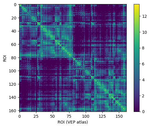
Load connectivity & one seizure:
conn = connectivity.Connectivity.from_file(f'{fsdir}/tvb/connectivity.vep.zip')
conn.configure()
conn.weights[:] = np.log(1 + conn.weights)
imshow(conn.weights); colorbar(); xlabel('ROI (VEP atlas)'), ylabel('ROI'); show();
2023-09-12 13:37:58,933 - WARNING - tvb.basic.readers - File 'hemispheres' not found in ZIP.
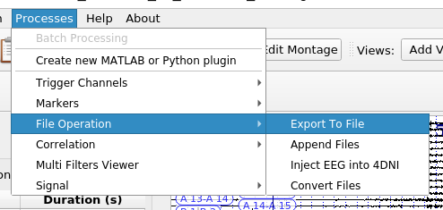
If seizure is not in VHDR, convert first with Anywave:
!ls ~/nextcloud/tutorial_data/Data_for_electrodes_labelling/Case1/SEEG
case1EEG_12HIP_RAS.TRC          case1EEG_13HIP_seizure.TRC.mrk
case1EEG_13HIP_seizure.TRC      case1EEG_13HIP_seizure.TRC.mtg
case1EEG_13HIP_seizure.TRC.bad      case1EEG_14HIP_seizure.TRC
case1EEG_13HIP_seizure.TRC.display
We open the TRC w/ Anywave, mark bad channels, isolate the section with the seizure with a marker for that section:
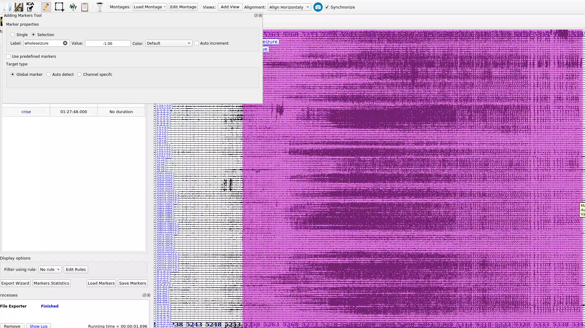
Start an export:
Set file name w/ marker name:
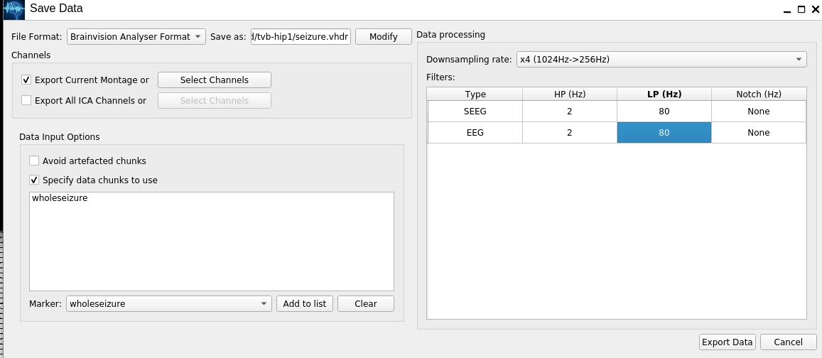
Save to the tvb folder, then load with MNE:
!ls ~/nextcloud/tvb-preprocessed-tutorial-data/fs/hip1/seeg/tvb-hip1
seizure-bipolar.eeg   seizure-monopolar.eeg   seizure.eeg
seizure-bipolar.vhdr  seizure-monopolar.vhdr  seizure.vhdr
seizure-bipolar.vmrk  seizure-monopolar.vmrk  seizure.vmrk
raw = mne.io.read_raw_brainvision(
    f'{fsdir}/seeg/tvb-hip1/seizure-bipolar.vhdr',
    preload=True
)
Extracting parameters from /home/woodman/nextcloud/tvb-preprocessed-tutorial-data/fs/hip1/seeg/tvb-hip1/seizure-bipolar.vhdr...
Setting channel info structure...
Reading 0 ... 25378  =      0.000 ...    99.133 secs...


/tmp/ipykernel_421/3985157263.py:1: RuntimeWarning: Limited 1 annotation(s) that were expanding outside the data range.
  raw = mne.io.read_raw_brainvision(
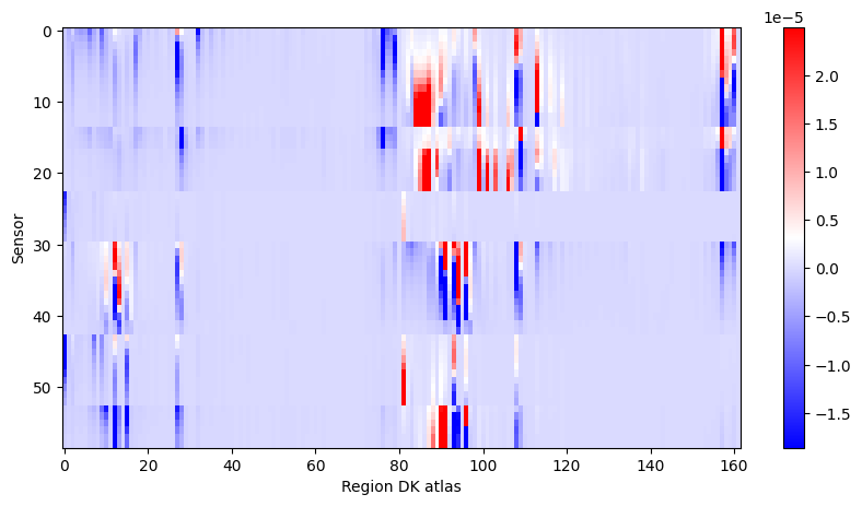
Construct gain matrix for bipolar electrodes in recording:
re_one = '([A-Z][A-Za-z]*\'?) ([0-9]+)'
re_bip = re.compile(f'{re_one}-{re_one}')
ch_bip_idx = []
bip_gain = []
electrodes = []
picks = []
pick_names = []
for i_ch, ch in enumerate(raw.ch_names):
    match = re_bip.match(ch)
    if match:
        picks.append(i_ch)
        pick_names.append(ch)
        e, i, _, j = match.groups()
        electrodes.append(e)
        i, j = int(i), int(j)
        e = e.replace('\'', 'p')
        ch_bip_idx.append((e, i, j))
        #pl_names.index(
        #r = np.sqrt(np.sum((cxyz(e,np.c_[i,j].T)[:,None] - conn.centres)**2, axis=2))
        try:
            cxyz = np.c_[pl_xyz[pl_names.index(f'{e}{i}')],
                         pl_xyz[pl_names.index(f'{e}{j}')]].T[:, None]
        except ValueError:
            pass
        r = np.sqrt(np.sum((cxyz - conn.centres)**2, axis=2))
        g = 1/r**3
        bip_gain.append(g[1] - g[0])
picks = np.array(picks)
bip_gain = np.array(bip_gain)
bip_gain = np.clip(bip_gain, *np.percentile(bip_gain.flat[:], [1,99]))
figure(figsize=(10, 5))
imshow(bip_gain, cmap='bwr', aspect='auto', interpolation='none'), colorbar(), xlabel('Region DK atlas'), ylabel('Sensor');
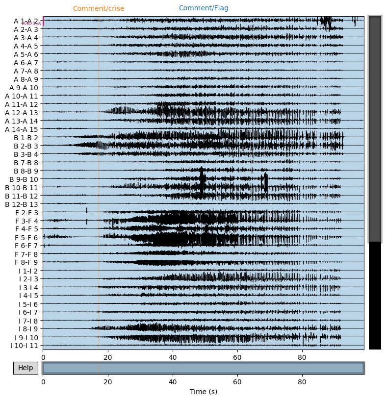
Pick out seizure from recording:
snip = raw.copy()
snip.pick_channels(pick_names)
snip.load_data()
snip.filter(1,30)
snip.resample(64)
snip.plot(n_channels=40,duration=100,scalings={'eeg':1e-3});
NOTE: pick_channels() is a legacy function. New code should use inst.pick(...).
Filtering raw data in 1 contiguous segment
Setting up band-pass filter from 1 - 30 Hz

FIR filter parameters
---------------------
Designing a one-pass, zero-phase, non-causal bandpass filter:
- Windowed time-domain design (firwin) method
- Hamming window with 0.0194 passband ripple and 53 dB stopband attenuation
- Lower passband edge: 1.00
- Lower transition bandwidth: 1.00 Hz (-6 dB cutoff frequency: 0.50 Hz)
- Upper passband edge: 30.00 Hz
- Upper transition bandwidth: 7.50 Hz (-6 dB cutoff frequency: 33.75 Hz)
- Filter length: 845 samples (3.301 s)

Using matplotlib as 2D backend.


[Parallel(n_jobs=1)]: Done  17 tasks      | elapsed:    0.0s
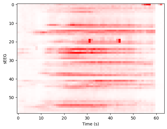
We construct the envelop of the data, per 1 s windows:
y, t = snip[:]
ysd = y[:,:y.shape[1]//64*64].reshape((len(y), 64, -1)).std(axis=-1)
scl = 1e-3
imshow(ysd, aspect='auto', interpolation='none', cmap='bwr', vmin=-scl, vmax=scl)
xlabel('Time (s)'), ylabel('sEEG'); show();
Projecting to TVB sources, we can determine a prior for the Epileptor x0 parameter based onset times:
ssd = np.clip(bip_gain.T.dot(ysd),0,1) * np.r_[1:0:64j]**3
x0p = ssd.sum(axis=-1)
x0p /= x0p.max()
x0p = -2.5 + x0p
figure(figsize=(8, 2)); plot(x0p); xlabel('ROI [LH, RH, subcort]'); ylabel('p(x0)'); show();
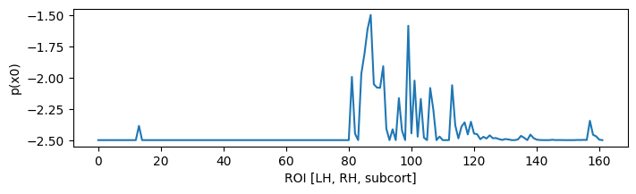
With a few examples for the ranking:
for i in np.argsort(x0p)[::-1][:5]:
    print(i, x0p[i], conn.region_labels[i])
87 -1.5 Right-Inferior-frontal-sulcus
99 -1.5861556255555924 Right-Precentral-sulcus-inferior-part
86 -1.6136127237070008 Right-F3-pars-opercularis
85 -1.8120990493471199 Right-F3-Pars-triangularis
91 -1.9098045348007213 Right-SFS-rostral
Now construct a simulation:
epileptor = models.Epileptor(Ks=np.r_[-0.2], Kf=np.r_[0.1], r=np.r_[0.00015])
epileptor.x0 = x0p
nsig = np.r_[0., 0., 0., 0.0005, 0.0005, 0.]
addnoise = noise.Additive(nsig=nsig, ntau=5.0)
initial = np.r_[-1.9, -17., 3.1, -1., 0.04, -0.17]
initial = np.zeros((100, 1, conn.number_of_regions, 1)) + initial[:, None, None]
sim = simulator.Simulator(
    connectivity=conn,
    coupling=coupling.Difference(a=np.r_[0.03]),
    model=epileptor,
    integrator=integrators.HeunStochastic(dt=0.05,noise=addnoise),
    initial_conditions=initial,
)
sim.configure()
Simulator: A Simulator assembles components required to perform simulations.
value |
|
|---|---|
Type |
Simulator |
conduction_speed |
3.0 |
connectivity |
Connectivity gid: b7b9f755-2761-4bc2-8115-ae8b475c11d2 |
coupling |
Difference gid: ba86c269-6714-4fe3-a7ae-7cce73061bc1 |
gid |
UUID(‘93b83c19-43a9-4da0-8a05-2d11e0756aa4’) |
initial_conditions |
[min, median, max] = [-17, -0.585, 3.1] dtype = float64 shape = (100, 6, 162, 1) |
integrator |
HeunStochastic gid: 17b17c7b-69ac-437e-81a1-18932deef33c |
model |
Epileptor gid: a883a1cb-d9f6-4e64-93e2-42d1347b40ef |
monitors |
(‘TemporalAverage’,) |
simulation_length |
1000.0 |
stimulus |
None |
surface |
None |
title |
Simulator gid: 93b83c19-43a9-4da0-8a05-2d11e0756aa4 |
Run the simulation:
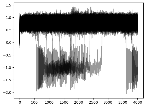
(t,y), = sim.run(simulation_length=4000.0)
y += randn(*y.shape)/10 # observation noise
Butterfly plot of source activity for seizure:
plot(t,y[:,0,:,0], 'k', alpha=0.4); show();
Projecting the source activity back to sources and creating an MNE Raw object from that, for analysis:
seeg = bip_gain.dot(y[:,0,:,0].T)
seeg /= seeg.std()
seeg *= snip[:][0].std()
info = mne.create_info(pick_names, 1e3/(t[1] - t[0])/8, 'eeg')
raw_sim = mne.io.RawArray(seeg, info)
raw_sim.info['sfreq']
Creating RawArray with float64 data, n_channels=59, n_times=4000
    Range : 0 ... 3999 =      0.000 ...    31.992 secs
Ready.


125.0
Then filter and inspect seizure:
raw_sim.filter(1,50,n_jobs=4)
raw_sim.plot(n_channels=40,duration=20,scalings={'eeg':2e-4});
Filtering raw data in 1 contiguous segment
Setting up band-pass filter from 1 - 50 Hz

FIR filter parameters
---------------------
Designing a one-pass, zero-phase, non-causal bandpass filter:
- Windowed time-domain design (firwin) method
- Hamming window with 0.0194 passband ripple and 53 dB stopband attenuation
- Lower passband edge: 1.00
- Lower transition bandwidth: 1.00 Hz (-6 dB cutoff frequency: 0.50 Hz)
- Upper passband edge: 50.00 Hz
- Upper transition bandwidth: 12.50 Hz (-6 dB cutoff frequency: 56.25 Hz)
- Filter length: 413 samples (3.304 s)


[Parallel(n_jobs=4)]: Using backend LokyBackend with 4 concurrent workers.
[Parallel(n_jobs=4)]: Done  14 tasks      | elapsed:    0.8s
[Parallel(n_jobs=4)]: Done  59 out of  59 | elapsed:    0.8s finished
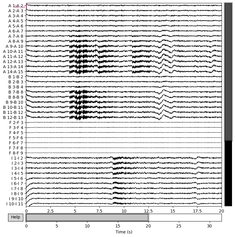
This shows that we can quickly reproduce a seizure similar the patient’s
with a TVB model, with an seizure onset heuristic. For a more precise
match, the x0 parameter of the model requires some tuning. This can
be done by hand or automatically, via Bayesian inference, which will be
the subject of another workflow example.