TUTORIALS
SEEG electrode placement with Brainstorm
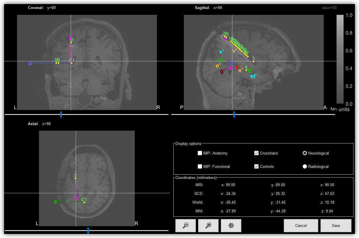
3D visualization of SEEG electrodes. SEEG electrodes have been generated and placed using Brainstorm .
Disclaimer
The methods and software used in this tutorial have not been certified for clinical practice and should be considered for research purposes only.
About this tutorial
The objective of this tutorial is to guide HIP users in placing SEEG electrodes on a post-implantation volume using Brainstorm. It primarily consists of a video demonstration and should be viewed as an introductory tutorial because it does not go into all the intricacies of the placement of SEEG electrodes.
For more in-depth information regarding the placement of SEEG electrodes using Brainstorm, please refer to the following official tutorials:
Requirements
There are no technical requirements to follow this tutorial because the dataset and software are available on the HIP.
HIP software used in this tutorial:
Brainstorm (07-Jan-2022)
HIP dataset used in this tutorial:
Epimap tutorial dataset (rev1.0)
Prepare the working environment
This tutorial relies on data available in the Epimap tutorial dataset, and the following file will be used:
anat/MRI/3DT1post_deface.nii
Copy this file into your private space so that it can be processed. Please, refer to the How to use the HIP spaces guide if you need help with this step. It is also advised to initiate a new Desktop. Pleases refer to the How to use Desktops and run applications from the App Catalog guide if you need help with this step.
Place SEEG electrodes with Brainstorm
Important
Applications running in a Desktop environment have access to your Private Space data under the /home/<HIP_USER>/nextcloud directory. Any data and/or configuration file outside of this directory will be lost when the application or desktop are closed. This is the only persistent directory as it is tied to the HIP user’s Private Space at application startup. Make sure you are always working within the /home/<HIP_USER>/nextcloud directory when using applications.
The accurate placement of SEEG electrodes requires some knowledge and a good understanding of the implantation procedure (an implantation scheme or equivalent) and of the type of material that has been implanted (SEEG electrode type/characteristics) and some expertise in brain anatomy. It is also important to work on a high-resolution CT scan or T1 MRI scan acquired after the implantation of the depth electrodes so that the recording contacts appear either in hypersignal or in hyposignal.
For confidentiality reasons, the implantation scheme will not be disclosed for this tutorial and the video demonstration focuses on the technical procedure to place SEEG electrodes and generate a standardized implantation file using Brainstorm.
SEEG electrode placement with 3D Slicer
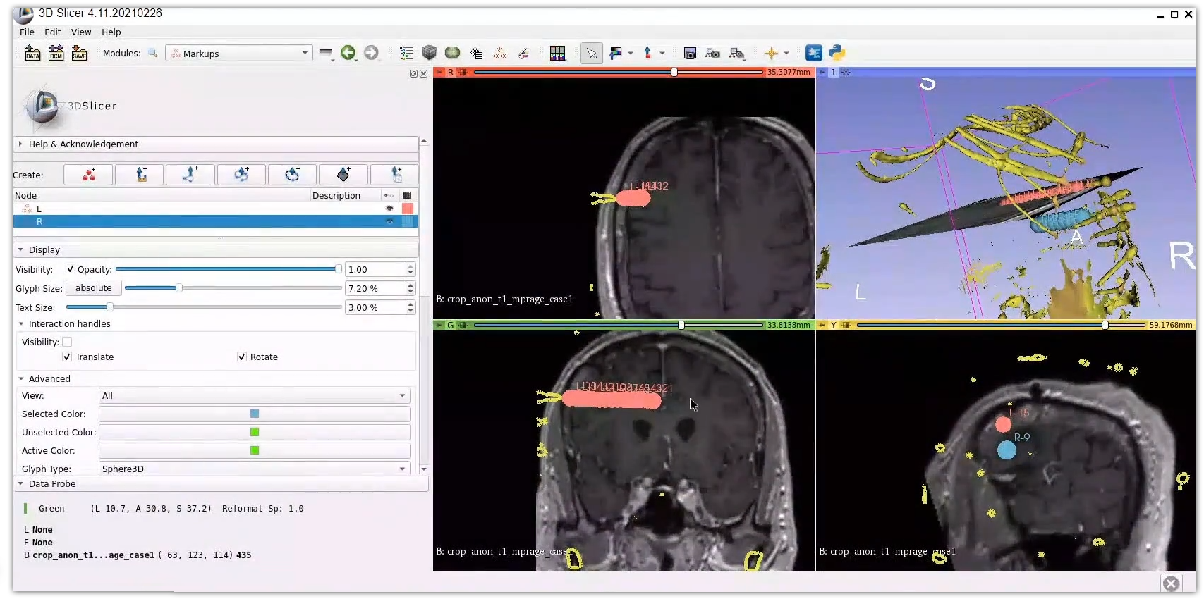
3D visualization of SEEG electrodes. SEEG electrodes have been generated and placed using 3D Slicer .
Disclaimer
The methods and software used in this tutorial have not been certified for clinical practice and should be considered for research purposes only.
About this tutorial
The objective of this tutorial is to guide HIP users in placing (non-rigid) SEEG electrodes on a post-implantation volume using 3D Slicer. It primarily consists of a video demonstration and should be viewed as an introductory tutorial because it does not go into all the intricacies of the placement of SEEG electrodes. For more in-depth information regarding electrode placement using 3D Slicer, please refer to the dedicated documentation.
Requirements
There are no technical requirements to follow this tutorial because the dataset and software are available on the HIP.
HIP softwares used in this tutorial:
HIP dataset used in this tutorial:
Data for electrodes labelling (rev1.0)
Prepare the working environment
This tutorial relies on data available in the dataset named Data for electrodes labelling, and the following folder has to be copied in your Private Space (this is demonstrated in the video tutorial):
/Data_for_electrodes_labelling/Case1
This tutorial requires to use several softwares, all available on the HIP, and it is advised to initiate a new Desktop. Please, refer to the How to use Desktops and run applications from the App Catalog guide if you need help with this step.
Place SEEG electrodes with 3D Slicer
Important
Applications running in a Desktop environment have access to your Private Space data under the /home/<HIP_USER>/nextcloud directory. Any data and/or configuration file outside of this directory will be lost when the application or desktop are closed. This is the only persistent directory as it is tied to the HIP user’s Private Space at application startup. Make sure you are always working within the /home/<HIP_USER>/nextcloud directory when using applications.
The accurate placement of SEEG electrodes requires some knowledge and a good understanding of the implantation procedure (an implantation scheme or equivalent) and of the type of material that has been implanted (SEEG electrode type/characteristics) and some expertise in brain anatomy. It is also important to work on a high-resolution CT scan or T1 MRI scan acquired after the implantation of the depth electrodes so that the recording contacts appear either in hypersignal or in hyposignal.
This video tutorial (19’30’’) relies on data publicly available on the HIP and desribes the different steps to label (non-rigid) SEEG electrodes, from the preparation of the imaging data using MRIcroGL and FSL, to the placement and exportation of SEEG contacts using 3D Slicer.
Epileptogenicity map computation with Brainstorm
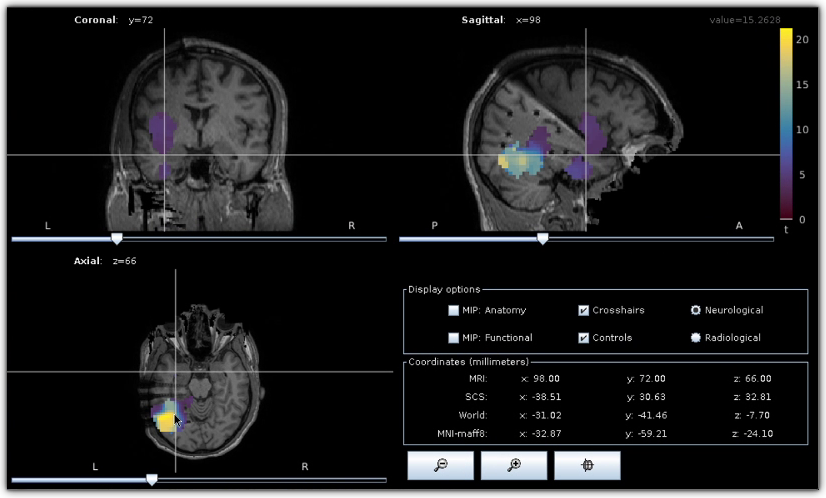
Epileptogenicity map. Epileptogenicity map computed and visualized using Brainstorm .
Disclaimer
The methods and software used in this tutorial have not been certified for clinical practice and should be considered for research purposes only.
About this tutorial
The objective of this tutorial is to guide HIP users in computing maps of epileptogenicity from ictal iEEG recordings. Epileptogenicity maps show the spatial distribution, and eventually the temporal evolution, of the Epileptogenicity Index (EI) in the subject’s brain. The EI is based on both spectral and temporal properties of iEEG signals and quantifies the presence of high-frequency oscillations also referred to rapid discharges. Rapid discharges have long been recognized as a characteristic electrophysiological pattern of the epileptogenic zone and can help identify brain regions generating seizures ([Bartolomei_2008]). This tutorial primarily consists of a video demonstration and should be viewed as an introductory tutorial because it does not go into all the intricacies of the computation of epileptogenicity maps.
For more in-depth information regarding the computation of epileptogenicity maps using Brainstorm, please refer to the official tutorial:
Requirements
There are no technical requirements to follow this tutorial because the dataset and software are available on the HIP.
HIP software used in this tutorial:
Brainstorm (07-Jan-2022)
HIP dataset used in this tutorial:
Epimap tutorial dataset (rev1.0)
Prepare the working environment
This tutorial relies on data available in the Epimap tutorial dataset, and the following files will be used:
anat/MRI/3DT1pre_deface.nii
anat/MRI/3DT1post_deface.nii
anat/implantation/elec_pos_patient.txt
seeg/SZ1.TRC
seeg/SZ2.TRC
seeg/SZ3.TRC
Copy those files into your private space so that they can be processed. Please, refer to the How to use the HIP spaces guide if you need help with this step. It is also advised to initiate a new Deskop. Please, refer to the How to use Desktops and run applications from the App Catalog guide if you need help with this step.
Compute a map of epileptogenicity
Important
Applications running in a Desktop environment have access to your Private Space data under the /home/<HIP_USER>/nextcloud directory. Any data and/or configuration file outside of this directory will be lost when the application or desktop are closed. This is the only persistent directory as it is tied to the HIP user’s Private Space at application startup. Make sure you are always working within the /home/<HIP_USER>/nextcloud directory when using applications.
It is mandatory to have the 3D positions of the recording contacts of the SEEG electrodes to compute epileptogenicity maps. The contact names and coordinates of the SEEG electrodes are provided in the elec_pos_patient.txt implantation file that will be used in this tutorial. If you work on your own imaging data and wish to generate a dedicated implantation file, you may want to look at the SEEG electrode placement with Brainstorm tutorial.
References
Bartolomei F, Chauvel P, Wendling F. Epileptogenicity of brain structures in human temporal lobe epilepsy: a quantified study from intracerebral EEG. Brain., 2008, 131(Pt 7):1818-30.
CCEP computation with Brainstorm
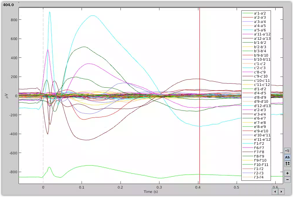
Visualization of CCEPs. The average response of a stimulation train was extracted from SEEG data using Brainstorm .
Disclaimer
The methods and software used in this tutorial have not been certified for clinical practice and should be considered for research purposes only.
About this tutorial
Electrical stimulation applied (sub)cortically can elicit CCEPs, recorded remotely from the stimulation site. The objective of this tutorial is to guide HIP users in computing the average response of a stimulation train extracted from a SEEG file using Brainstorm. It primarily consists of a video demonstration and should be viewed as an introductory tutorial because it does not go into all the intricacies of the processing steps used to compute CCEPs.
For more in-depth information regarding some of the processing steps illustrated in the video, please refer to the following official tutorials:
Requirements
There are no technical requirements to follow this tutorial because the dataset and software are available on the HIP.
HIP software used in this tutorial:
Brainstorm (07-Jan-2022)
HIP dataset used in this tutorial:
“CCEP tutorial dataset” located in the shared tutorial_data folder.
Prepare the working environment
This tutorial relies on data available in the “CCEP tutorial dataset” located in the read-only shared folder called tutorial_data, and the following file has to be copied in your Private Space (this is demonstrated in the video tutorial):
sub-anon_task-stimulation_run-01.edf
This tutorial requires to use Brainstorm, which is available on the HIP, and it is advised to initiate a new Desktop. Please, refer to the How to use Desktops and run applications from the App Catalog guide if you need help with this step.
Compute cortico-cortical evoked potentials
Important
Applications running in a Desktop environment have access to your Private Space data under the /home/<HIP_USER>/nextcloud directory. Any data and/or configuration file outside of this directory will be lost when the application or desktop are closed. This is the only persistent directory as it is tied to the HIP user’s Private Space at application startup. Make sure you are always working within the /home/<HIP_USER>/nextcloud directory when using applications.
There are different ways to compute CCEPs depending on your data and the analyzes you want to perform. The processing steps used in this tutorial are derived from a pipeline developed during The Functional Brain Tractography Project (see [Trebaul_2018c] for full scientific details) which has been simplified for demonstration purposes. Notably, this tutorial shows how to: (1) import raw SEEG data into Brainstorm; (2) extract a stimulation train; (3) mark bad channels; (4) detect the stimulation artifacts (individual pulses); (5) apply bipolar montage; (6) remove stimulation artifacts; (7) apply a band-pass filter; (8) compute the average response across all pulses. Depending on your objective, some of these steps might not be relevant/necessary or might be executed in a different order.
This video tutorial (14’04’’) relies on data publicly available on the HIP and describes the different steps to compute CCEPs using Brainstorm:
References
Trebaul, L., Deman, P., Tuyisenge, V., Jedynak, M., Hugues, E., Rudrauf, D., Bhattacharjee, M., Tadel, F., Chanteloup-Forêt, B., Saubat, C., Reyes Mejia, G.C., Adam, C., Nica, A., Pail, M., Dubeau, F., Rheims, S., Trébuchon, A., Wang, H., Liu, S., Blauwblomme, T., Garces, M., De Palma, L., Valentín, A., Metsahonkala, E.-L., Petrescu, A.M., Landré, E., Szurhaj, W., Hirsch, E., Valton, L., Rocamora, R., Schulze-Bonhage, A., Mîndruţă, I., Francione, S., Maillard, L., Taussig, D., Kahane, P., David, O., 2018. Probabilistic functional tractography of the human cortex revisited. NeuroImage 181, 414–429. doi:10.1016/j.neuroimage.2018.07.039.
Warning
The tutorial is still in the process of being finalized.
Simulation workflow with The Virtual Brain
Disclaimer
The methods and software used in this tutorial have not been certified for clinical practice and should be considered for research purposes only.
Requirements
There are no technical requirements to follow this tutorial because the dataset and software are available on the HIP.
HIP software used in this tutorial:
HIP dataset used in this tutorial:
“tvb-preprocessed-tutorial-data” located in the shared tutorial_data folder.
Prepare the working environment
This tutorial requires to use The Virtual Brain, which is available on the HIP, and it is advised to initiate a new Desktop. Please, refer to the How to use Desktops and run applications from the App Catalog guide if you need help with this step.
Simulation workflow
Jupyter Notebook
Once The Virtual Brain app has started, you can view this tutorial in the form of an interactive Jupyter Notebook by double clicking the file named “simulation.ipynb” in the left sidebar.
Here we will show a short demonstration of using data from HIP partners to do simulation, with parameters guessed from one of the patient’s seizures.
%pylab inline
import re
import numpy as np
import mne
import nibabel
from tvb.simulator.lab import *
%pylab is deprecated, use %matplotlib inline and import the required libraries.
Populating the interactive namespace from numpy and matplotlib

/usr/local/lib/python3.10/dist-packages/tvb/datatypes/surfaces.py:60: UserWarning: Geodesic distance module is unavailable; some functionality for surfaces will be unavailable.
  warnings.warn(msg)
Let’s check our access to some data.
First sEEG contacts: use your favorite 3D tool to localize sEEG contacts in T1 space as in the following example:
!head ~/nextcloud/tvb-preprocessed-tutorial-data/fs/hip1/elec/seeg.xyz
L1      -12.20   53.60   67.20
L2       -8.70   53.65   67.20
L3       -5.20   53.69   67.20
L4       -1.70   53.74   67.20
L5        1.80   53.78   67.20
L6        5.30   53.83   67.20
L7        8.80   53.88   67.20
L8       12.30   53.92   67.20
L9       15.80   53.97   67.20
L10      19.30   54.02   67.20
Then we load them:
pl_names = []
pl_xyz = []
fsdir = os.path.expanduser('~/nextcloud/tvb-preprocessed-tutorial-data/fs/hip1')
with open(f'{fsdir}/elec/seeg.xyz', 'r') as fd:
    for line in fd.readlines():
        if line.startswith('plot'):
            continue
        name, *xyz = [_ for _ in line.strip().split(' ') if _.strip()]
        pl_names.append(name)
        pl_xyz.append(np.array([float(_) for _ in xyz]))
Load connectivity & one seizure:
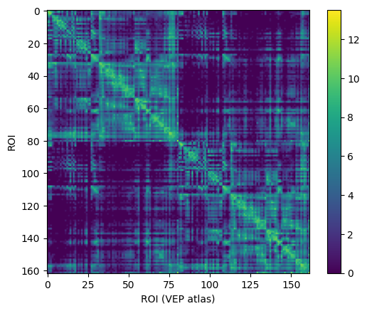
conn = connectivity.Connectivity.from_file(f'{fsdir}/tvb/connectivity.vep.zip')
conn.configure()
conn.weights[:] = np.log(1 + conn.weights)
imshow(conn.weights); colorbar(); xlabel('ROI (VEP atlas)'), ylabel('ROI'); show();
2023-09-12 13:37:58,933 - WARNING - tvb.basic.readers - File 'hemispheres' not found in ZIP.
If seizure is not in VHDR, convert first with Anywave:
!ls ~/nextcloud/tutorial_data/Data_for_electrodes_labelling/Case1/SEEG
case1EEG_12HIP_RAS.TRC          case1EEG_13HIP_seizure.TRC.mrk
case1EEG_13HIP_seizure.TRC      case1EEG_13HIP_seizure.TRC.mtg
case1EEG_13HIP_seizure.TRC.bad      case1EEG_14HIP_seizure.TRC
case1EEG_13HIP_seizure.TRC.display
We open the TRC w/ Anywave, mark bad channels, isolate the section with the seizure with a marker for that section:
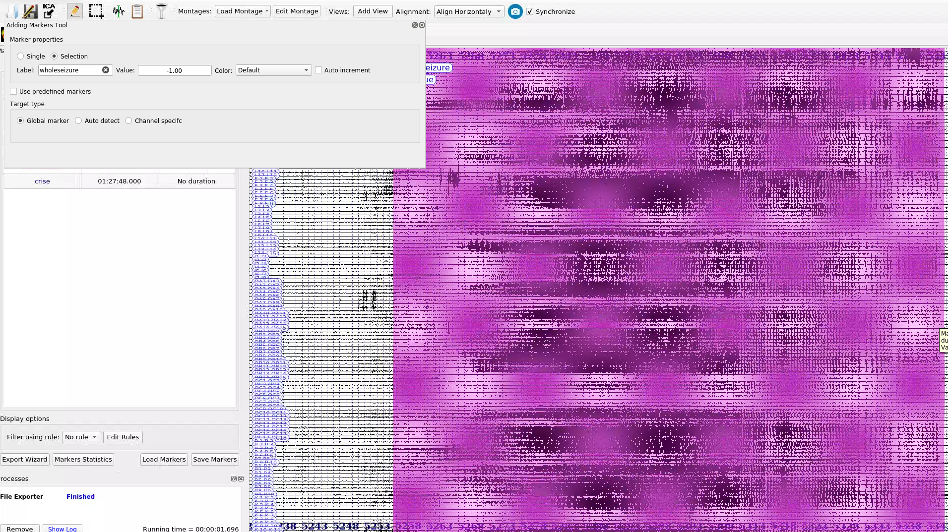
Start an export:
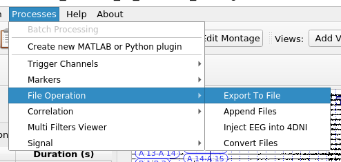
Set file name w/ marker name:
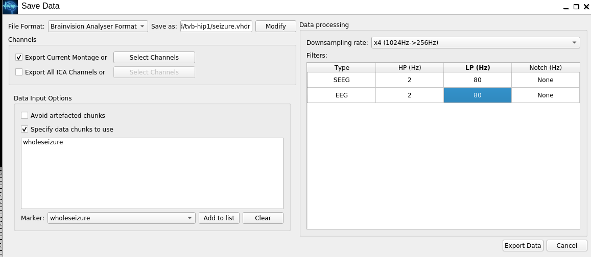
Save to the tvb folder, then load with MNE:
!ls ~/nextcloud/tvb-preprocessed-tutorial-data/fs/hip1/seeg/tvb-hip1
seizure-bipolar.eeg   seizure-monopolar.eeg   seizure.eeg
seizure-bipolar.vhdr  seizure-monopolar.vhdr  seizure.vhdr
seizure-bipolar.vmrk  seizure-monopolar.vmrk  seizure.vmrk
raw = mne.io.read_raw_brainvision(
    f'{fsdir}/seeg/tvb-hip1/seizure-bipolar.vhdr',
    preload=True
)
Extracting parameters from /home/woodman/nextcloud/tvb-preprocessed-tutorial-data/fs/hip1/seeg/tvb-hip1/seizure-bipolar.vhdr...
Setting channel info structure...
Reading 0 ... 25378  =      0.000 ...    99.133 secs...


/tmp/ipykernel_421/3985157263.py:1: RuntimeWarning: Limited 1 annotation(s) that were expanding outside the data range.
  raw = mne.io.read_raw_brainvision(
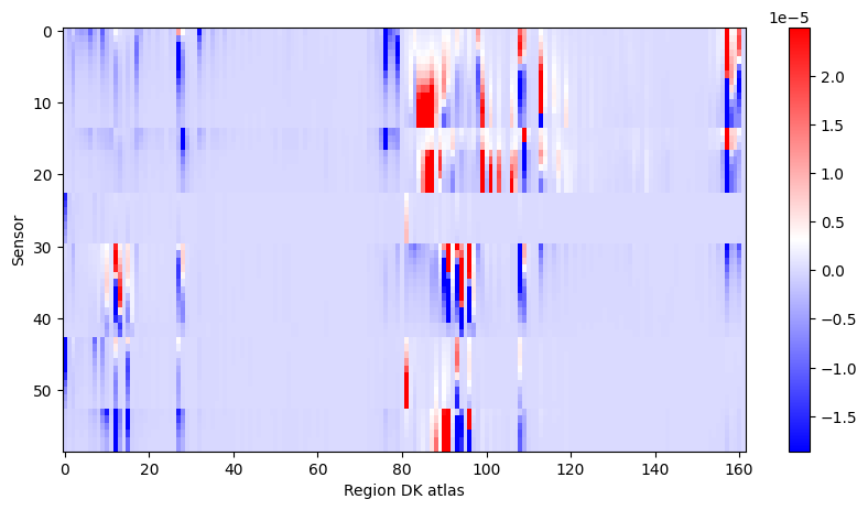
Construct gain matrix for bipolar electrodes in recording:
re_one = '([A-Z][A-Za-z]*\'?) ([0-9]+)'
re_bip = re.compile(f'{re_one}-{re_one}')
ch_bip_idx = []
bip_gain = []
electrodes = []
picks = []
pick_names = []
for i_ch, ch in enumerate(raw.ch_names):
    match = re_bip.match(ch)
    if match:
        picks.append(i_ch)
        pick_names.append(ch)
        e, i, _, j = match.groups()
        electrodes.append(e)
        i, j = int(i), int(j)
        e = e.replace('\'', 'p')
        ch_bip_idx.append((e, i, j))
        #pl_names.index(
        #r = np.sqrt(np.sum((cxyz(e,np.c_[i,j].T)[:,None] - conn.centres)**2, axis=2))
        try:
            cxyz = np.c_[pl_xyz[pl_names.index(f'{e}{i}')],
                         pl_xyz[pl_names.index(f'{e}{j}')]].T[:, None]
        except ValueError:
            pass
        r = np.sqrt(np.sum((cxyz - conn.centres)**2, axis=2))
        g = 1/r**3
        bip_gain.append(g[1] - g[0])
picks = np.array(picks)
bip_gain = np.array(bip_gain)
bip_gain = np.clip(bip_gain, *np.percentile(bip_gain.flat[:], [1,99]))
figure(figsize=(10, 5))
imshow(bip_gain, cmap='bwr', aspect='auto', interpolation='none'), colorbar(), xlabel('Region DK atlas'), ylabel('Sensor');
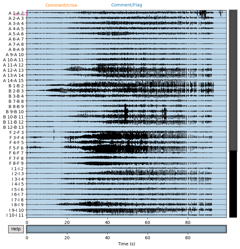
Pick out seizure from recording:
snip = raw.copy()
snip.pick_channels(pick_names)
snip.load_data()
snip.filter(1,30)
snip.resample(64)
snip.plot(n_channels=40,duration=100,scalings={'eeg':1e-3});
NOTE: pick_channels() is a legacy function. New code should use inst.pick(...).
Filtering raw data in 1 contiguous segment
Setting up band-pass filter from 1 - 30 Hz

FIR filter parameters
---------------------
Designing a one-pass, zero-phase, non-causal bandpass filter:
- Windowed time-domain design (firwin) method
- Hamming window with 0.0194 passband ripple and 53 dB stopband attenuation
- Lower passband edge: 1.00
- Lower transition bandwidth: 1.00 Hz (-6 dB cutoff frequency: 0.50 Hz)
- Upper passband edge: 30.00 Hz
- Upper transition bandwidth: 7.50 Hz (-6 dB cutoff frequency: 33.75 Hz)
- Filter length: 845 samples (3.301 s)

Using matplotlib as 2D backend.


[Parallel(n_jobs=1)]: Done  17 tasks      | elapsed:    0.0s
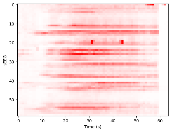
We construct the envelop of the data, per 1 s windows:
y, t = snip[:]
ysd = y[:,:y.shape[1]//64*64].reshape((len(y), 64, -1)).std(axis=-1)
scl = 1e-3
imshow(ysd, aspect='auto', interpolation='none', cmap='bwr', vmin=-scl, vmax=scl)
xlabel('Time (s)'), ylabel('sEEG'); show();
Projecting to TVB sources, we can determine a prior for the Epileptor x0 parameter based onset times:
ssd = np.clip(bip_gain.T.dot(ysd),0,1) * np.r_[1:0:64j]**3
x0p = ssd.sum(axis=-1)
x0p /= x0p.max()
x0p = -2.5 + x0p
figure(figsize=(8, 2)); plot(x0p); xlabel('ROI [LH, RH, subcort]'); ylabel('p(x0)'); show();
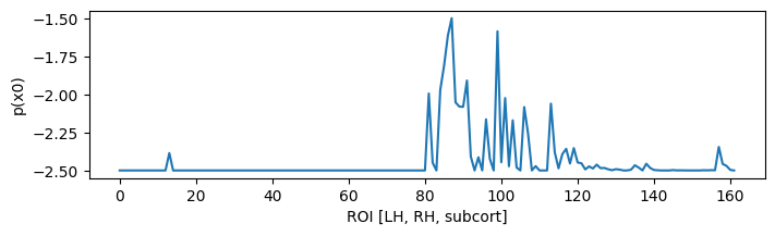
With a few examples for the ranking:
for i in np.argsort(x0p)[::-1][:5]:
    print(i, x0p[i], conn.region_labels[i])
87 -1.5 Right-Inferior-frontal-sulcus
99 -1.5861556255555924 Right-Precentral-sulcus-inferior-part
86 -1.6136127237070008 Right-F3-pars-opercularis
85 -1.8120990493471199 Right-F3-Pars-triangularis
91 -1.9098045348007213 Right-SFS-rostral
Now construct a simulation:
epileptor = models.Epileptor(Ks=np.r_[-0.2], Kf=np.r_[0.1], r=np.r_[0.00015])
epileptor.x0 = x0p
nsig = np.r_[0., 0., 0., 0.0005, 0.0005, 0.]
addnoise = noise.Additive(nsig=nsig, ntau=5.0)
initial = np.r_[-1.9, -17., 3.1, -1., 0.04, -0.17]
initial = np.zeros((100, 1, conn.number_of_regions, 1)) + initial[:, None, None]
sim = simulator.Simulator(
    connectivity=conn,
    coupling=coupling.Difference(a=np.r_[0.03]),
    model=epileptor,
    integrator=integrators.HeunStochastic(dt=0.05,noise=addnoise),
    initial_conditions=initial,
)
sim.configure()
Simulator: A Simulator assembles components required to perform simulations.
value |
|
|---|---|
Type |
Simulator |
conduction_speed |
3.0 |
connectivity |
Connectivity gid: b7b9f755-2761-4bc2-8115-ae8b475c11d2 |
coupling |
Difference gid: ba86c269-6714-4fe3-a7ae-7cce73061bc1 |
gid |
UUID(‘93b83c19-43a9-4da0-8a05-2d11e0756aa4’) |
initial_conditions |
[min, median, max] = [-17, -0.585, 3.1] dtype = float64 shape = (100, 6, 162, 1) |
integrator |
HeunStochastic gid: 17b17c7b-69ac-437e-81a1-18932deef33c |
model |
Epileptor gid: a883a1cb-d9f6-4e64-93e2-42d1347b40ef |
monitors |
(‘TemporalAverage’,) |
simulation_length |
1000.0 |
stimulus |
None |
surface |
None |
title |
Simulator gid: 93b83c19-43a9-4da0-8a05-2d11e0756aa4 |
Run the simulation:
(t,y), = sim.run(simulation_length=4000.0)
y += randn(*y.shape)/10 # observation noise
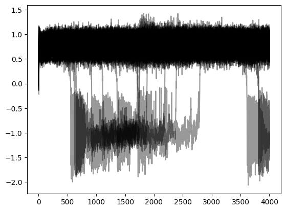
Butterfly plot of source activity for seizure:
plot(t,y[:,0,:,0], 'k', alpha=0.4); show();
Projecting the source activity back to sources and creating an MNE Raw object from that, for analysis:
seeg = bip_gain.dot(y[:,0,:,0].T)
seeg /= seeg.std()
seeg *= snip[:][0].std()
info = mne.create_info(pick_names, 1e3/(t[1] - t[0])/8, 'eeg')
raw_sim = mne.io.RawArray(seeg, info)
raw_sim.info['sfreq']
Creating RawArray with float64 data, n_channels=59, n_times=4000
    Range : 0 ... 3999 =      0.000 ...    31.992 secs
Ready.


125.0
Then filter and inspect seizure:
raw_sim.filter(1,50,n_jobs=4)
raw_sim.plot(n_channels=40,duration=20,scalings={'eeg':2e-4});
Filtering raw data in 1 contiguous segment
Setting up band-pass filter from 1 - 50 Hz

FIR filter parameters
---------------------
Designing a one-pass, zero-phase, non-causal bandpass filter:
- Windowed time-domain design (firwin) method
- Hamming window with 0.0194 passband ripple and 53 dB stopband attenuation
- Lower passband edge: 1.00
- Lower transition bandwidth: 1.00 Hz (-6 dB cutoff frequency: 0.50 Hz)
- Upper passband edge: 50.00 Hz
- Upper transition bandwidth: 12.50 Hz (-6 dB cutoff frequency: 56.25 Hz)
- Filter length: 413 samples (3.304 s)


[Parallel(n_jobs=4)]: Using backend LokyBackend with 4 concurrent workers.
[Parallel(n_jobs=4)]: Done  14 tasks      | elapsed:    0.8s
[Parallel(n_jobs=4)]: Done  59 out of  59 | elapsed:    0.8s finished
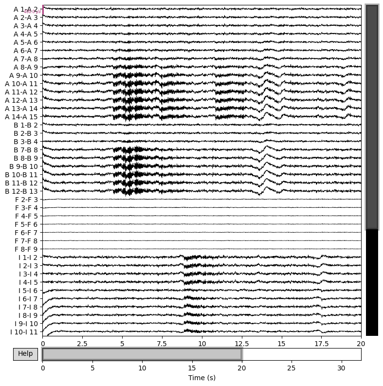
This shows that we can quickly reproduce a seizure similar the patient’s
with a TVB model, with an seizure onset heuristic. For a more precise
match, the x0 parameter of the model requires some tuning. This can
be done by hand or automatically, via Bayesian inference, which will be
the subject of another workflow example.